The Stratified Cox Procedure

---

Introduction

Definition

The stratified cox model is a modification of the cox proportional hazards (PH) model that allows for control by stratification of a predictor that does not satisfy by the PH assumption. Predictors that are assumed to satisfy the PH assumption are included in the model, whereas the predictor being stratified is not included.

Example

These are the computer results for a Cox PH model that includes three variables - log WBC, treatment group $(R_x)$, and SEX - from a clinical trial of 42 leukemia patients. The goal of the trial was to determine the number of days patients remained in remission.

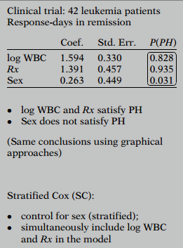
The P(PH) values for logWBC and treatment group were found to be non-significant, but the P(PH) value for SEX was significant at a level at 0.05. This suggests that logWBC and treatment group conform to the PH assumption, while SEX does not. These findings were supported by the graphical procedures discussed earlier.

As one of the predictors did not meet the PH assumption, we performed a stratified Cox (SC) procedure for analysis. This allowed us to control for the variable that did not meet the PH assumption (SEX) by stratification, while including the logWBC and treatment variables that did meet the PH assumption in the model.

---

The General Stratified Cox(SC) Model

We assume that we have $k$ variables not satisfying the PH assumption and $p$ variables satisfying the PH assumption. The variables not satisfying the PH assumption we denote as $Z_1, Z_2,\cdots, Z_k$; the variables satisfying the PH assumption we denote as $X_1, X_2,\cdots, X_p$.

To perform the stratified Cox procedure, we define a single new variable, which we call $Z^*$, from the $Z$'s to be used for stratification. We do this by forming categories of each $Z_i$, including those $Z_i$ that are interval variables. We then form combinations of categories, and these combinations are our strata. These strata are the categories of the new variable $Z^*$.

For example, suppose $k$ is 2, and the two $Z$'s are age (an interval variable) and treatment status (a binary variable). Then we categorize age into, say, three age groups - young, middle, and old. We then form six age group-by-treatment status combinations, as shown here. These six combinations represent the different categories of a single new variable that we stratify on in our stratified Cox model. We call this new variable $Z^*$.

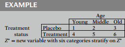
In general, the stratification variable $Z^*$ will have $k^*$ categories, where $k^*$ is the total number of combinations (or strata) formed after categorizing each of the $Z$'s. In the above example, $k^*$ is equal to 6.

We now present the general hazard function form for the stratified Cox model, as shown here. This formula contains a subscript g which indicates the $g$-th stratum. The strata are defined as the different categories of the stratification variable $Z^*$, and the number of strata equals $k^*$.

The general SC model:

$$h_g(t,\mathbf{X})=h_{0g}(t)e^{\beta_1X_1+\beta_2X_2+\cdots+\beta_pX_p}$$

$$g=1,2,\cdots,k^*, \text{strata defined from Z*}$$

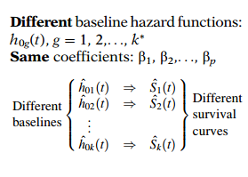
Note that the variable $Z^*$ is not explicitly included in the model but that the $X$'s, which are assumed to satisfy the PH assumption, are included in the model.

Note also that the baseline hazard function $h_{0g}(t)$ is allowed to be different for each stratum. However, the coefficients $\beta_1, \beta_2,..., \beta_p$ are the same for each stratum.

---

A Graphical View of the Stratified Cox Approach

In this section we examine four log-log survival plots illustrating the assumptions underlying a stratified Cox model with or without interaction. Each of the four models considers two dichotomous predictors: treatment (coded $R_X = 1$ for placebo and $R_X = 0$ for new treatment) and SEX (coded 0 for females and 1 for males). The four models are as follows.

1. This model assumes the PH assumption for both RX and SEX and also assumes no interaction between RX and SEX. Notice all four log-log curves are parallel (PH assumption) and the effect of treatment is the same for females and males (no interaction). The effect of treatment (controlling for SEX) can be interpreted as the distance between the log-log curves from $R_X = 1$ to $R_X = 0$, for males and for females, separately.

   $$h(t)=h_0(t)e^{\beta_1R_X+\beta_2\text{SEX}}$$
   $$\mathrm{ln}({-\mathrm{ln}S(t)})=\mathrm{ln}({-\mathrm{ln}S_0(t)})+\beta_1R_X+\beta_2\text{SEX}$$
   

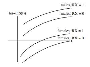
2. This model assumes the PH assumption for both RX and SEX and allows for interaction between these two variables. All four log-log curves are parallel (PH assumption) but the effect of treatment is larger for males than females as the distance from $R_X = 1$ to $R_X = 0$ is greater for males.

   $$h(t)=h_0(t)e^{\beta_1R_X+\beta_2\text{SEX}+\beta_3R_X\times\text{SEX}}$$
   $$\mathrm{ln}({-\mathrm{ln}S(t)})=\mathrm{ln}({-\mathrm{ln}S_0(t)})+\beta_1R_X+\beta_2\text{SEX}+\beta_3R_X\times\text{SEX}$$
   

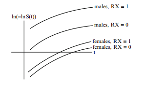
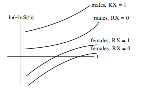
3. This is a stratified Cox model in which the PH assumption is not assumed for SEX. Notice the curves for males and females are not parallel. However, the curves for RX are parallel within each stratum of SEX indicating that the PH assumption is satisfied for RX. The distance between the log-log curves from $R_X = 1$ to $R_X = 0$ is the same for males and females indicating no interaction between $R_X$ and SEX.

   $$h(t)=h_{0g}(t)e^{\beta_1R_X}$$

   (g = 1 for males, g = 0 for females)

   $$\mathrm{ln}({-\mathrm{ln}S(t)})=\mathrm{ln}({-\mathrm{ln}S_{0g}(t)})+\beta_1R_X$$
   

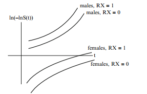
4. This is a stratified Cox model allowing for interaction of RX and SEX. The curves for males and females are not parallel although the PH assumption is satisfied for RX within each stratum of SEX.The distance between the log-log curves from $R_X = 1$ to $R_X= 0$ is greater for males than females indicating interaction between RX and SEX.

   $$h(t)=h_{0g}(t)e^{\beta_1R_X+\beta_2R_X\times \text{SEX}}$$

   (g = 1 for males, g = 0 for females)

   $$\mathrm{ln}({-\mathrm{ln}S(t)})=\mathrm{ln}({-\mathrm{ln}S_{0g}(t)})+\beta_1R_X++\beta_2R_X\times \text{SEX}$$